Options & Volatility

Roughly a week ago, we witnessed the second-largest liquidation event in Deribit history. Doing some research, it seems that the rapid liquidation of these short positions was one of the driving factors in the 10% drawdown.

This piqued my curiosity, and I started diving into the rabbit hole of the options abyss...

One concept important to options is volatility. Which makes you wonder, what is volatility and how does an options exchange like Deribit calculate it?

In this post, I will share my learnings on volatility, how to calculate it using historical prices, and also how I approach this using my software engineering brain. Also, for many of the options, I make references to a useful options resource Dynamic Hedging: Managing Vanilla and Exotic Options. You purchase the book online (there's a PDF version as well but I am not sharing it here).

Defining Volatility

In our case, we won't be looking at Implied Volatility (this is a separate blog post for another day) but Actual Volatility (also known as Historical Volatility or Realized Volatility).

In layman's terms, volatility is used to measure how wide the price swings for an asset. The higher the volatility, the larger we typically expect the asset prices to swing.

Volatility is best defined as the amount of variability in the returns of an asset. Actual Volatility is the actual movement experienced by the market

Knowing this, we can use a more mathematical way of defining this. Since we are measuring the swings in the prices, a good statistical measure would be to use the variance \(\sigma^2_x\) or the standard deviation \(\sigma_x\).

Calculating using deviation from mean

As we all learnt in stats class, standard deviation is calculated using the following formula:

$$\sigma_x = \sqrt{\frac{1}{n-1}\sum_{t=1}^n{(x_t-\bar{x})^2}} \space$$

$$\bar{x} = \sum_{t=1}^n{\frac{x_t}{n}}$$

Given a time series data of prices, we just need to:

1. Find the mean of the prices \(\bar{x}\).

2. For each price data point, find the deviation from the mean

3. Get the variance \(\sigma^2_x\) by taking the sum of squares and dividing it by \(n\) (minus delta degrees of freedom)

4. Finally, to get the standard deviation \(\sigma_x\), just square root it!

Easy and simple! Python already has an out-of-the-box function for it called np.std. This function essentially does the above by running the following std = sqrt(mean(abs(a - a.mean())**2))

In our case, we will have to implement the standard deviation calculation by ourselves for a very obvious reason (you will find out later). Implementing from scratch isn't too hard anyways, in my case, I create a function calculate_vols that takes in a DataFrame and uses a rolling window to calculate it.

To get the results, we can do the following calculate_vols(df=dataset, window_size=7, ddof=1) and vary the window_size accordingly.

def calculate_vols(df: pd.DataFrame, window_size: int, ddof: int) -> pd.DataFrame:
    res = df.copy()
    res['avg'] = res['Close'].rolling(window=window_size).mean()
    res['deviation'] = (res['Close'] - res['avg'])/res['Close']
    res['squared'] = np.square(res['deviation'])
    res['sum'] = res['squared'].rolling(window=window_size).sum()
    res['variance'] = res['sum']/(window_size-ddof)
    res['std-dev'] = np.sqrt(res['variance'])

    res['vol'] = res['std-dev']*annualize
    return res[window_size:]

If we have a variable length time-series dataset, the rolling window allows us to calculate the 7-day, 14-day or even 30-day standard deviation. For example, we can use a 2-year time-series dataset to calculate the 7-day, 30-day, 90-day and 180-day volatility like how Deribit needs.

Calculating using Log Returns

Why use Log Returns?

In finance, volatility is calculated by measuring price movements(price today vs price yesterday) instead of deviations from the mean(price today vs mean price). At first glance, this seems puzzling - why do we deviate from the typical way of measuring standard deviation?

There's a very strong and valid reason for this. Quoting from Nassim Taleb's book (earlier),

If a market moved 1% a day every day in the same direction (say upward) for an entire month, the conventional measurement of volatility would put it at 0% since all of the moves were at the mean move. This clashes with an option trader's instinct. An option trader would still consider it to be 1% a day and in this case would prefer to buy volatility when it is offered cheaper than 16%.

Simply put, if an asset moves by x%, we would like to measure volatility with the price movement itself and not the difference from the mean. Averages can and in fact, be very deceiving since they can become a lagging indicator!

$$x_t = \log(\frac{P_t}{P_{t-1}})$$

$$\sigma'x=\sqrt{\frac{1}{n}\sum_{t=1}^n{x_t^2}} \space$$

Logarithm transformations also have very unique properties. Being primarily a software engineer, I filtered the following essentials:

• Approximation: The (natural) log is roughly equal to the percentage return especially when it is close to 0. So we can take the log returns as such an approximation.

• Accumulator: Log returns are additive in nature, this means we can sum the log returns over a period to measure cumulative returns. This unique property of logarithms is not just limited to here (this unique mathematical property has optimization benefits - look at reducing gas cost geometric calculations in smart contracts!)

Implementing it...

We can change calculate_vols to inject a function to calculate the deviation.

def calculate_vols(df: pd.DataFrame, window_size: int,  ddof: int, deviationFn: callable,) -> pd.DataFrame:
    res = df.copy()
    res['deviation'] = deviationFn(res, window_size)
    res['squared'] = np.square(res['deviation'])
    res['sum'] = res['squared'].rolling(window=window_size).sum()
    res['variance'] = res['sum']/(window_size-ddof)
    res['std-dev'] = np.sqrt(res['variance'])

    res['vol'] = res['std-dev']*annualize
    return res[window_size:]

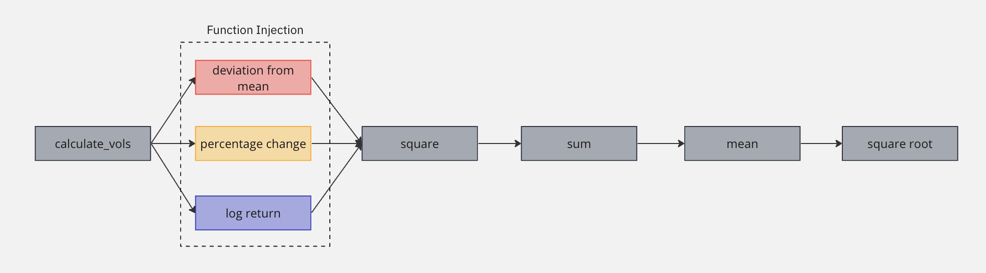
To calculate this, let's create a custom deviationFn that takes the log returns

def deviationFn(x: pd.DataFrame, window_size: int):
    return np.log(x['Close']/x['Close'].shift(1))

To get the volatility, simply run calculate_vols with a delta degree of freedom (ddof) of 0 since we are no longer using the mean: calculate_vols(df=dataset, window_size=30, ddof=0, deviationFn=deviationFn)

With the new and improved calculate_vols(), we can adjust the deviationFn to calculate volatility using the deviation from mean.

def deviationFn(x: pd.DataFrame, window_size: int):
    x['avg'] = x['Close'].rolling(window=window_size).mean()
    return (x['Close'] - x['avg'])/x['Close']

Or even just the percentage change of returns.

def deviationFn(x: pd.DataFrame, window_size: int):
    return x['Close'].diff()/x['Close']

End

Thank you for sticking to the end and hope you have learnt more about volatility and standard deviation! I am also planning to learn and cover beta & correlations (for pair trading) and maybe Implied Volatility and Deribit's DVOL! I will slowly add it into my github repo implementation here:

There are also other ways to calculate actual volatility such as the Parkinsons volatility with the following formula:

$$P=\sqrt{\frac{1}{n} \sum_{i=1}^n{\frac{1}{4\log2}} \left[\log\frac{S_H}{S_L}\right]^2}$$

I shall leave the implementation of this to you as it is way too complex for a simple blog post like this haha.